Processing Multi-Spectral UAS imagery For Value Added Data Analysis

Introduction

The RedEdge sensor is a multispectral camera that can capture five distinguishable spectral bands to generate precise and quantitative information on the vigor and health of crops. These 5 spectral bands include Blue, Green, Red, Red Edge, and Near Infrared (NIR). Some of the specs on the RedEdge sensor includes a 1 capture per second of all bands, 8.2 cm/pixel at 120 m AGL, 150 grams, and powered by 5.0 volts. The RedEdge sensor can provide much greater detail when it comes to imagery over the Red, Green, and Blue (RGB) sensor. This includes using the RedEdge sensor to gain a greater understanding specific agricultural areas of interest to study.

Methods

Copying data in this lab included making a new folder to store all of the RedEdge imagery and any further information or maps that are created throughout this lab. This folder will be used when processing the RedEdge imagery.

Next step is to process the Imagery in Pix4D that was copied over into the specified folder. When creating the new project, make sure to select the “Ag-Multispectral”(figure 1) template rather than the 3D template like what we had used in the previous labs. When opening the processing options, select all the necessary options shown in figure 2. Once all the correct options are selected, processing can begin. This imagery will take longer to process than the previous labs did.

Figure 1. Ag Multispectral processing template is selected for value added data analysis

 Figure 2. Processing options dialog box

After the imagery is done processing, the next step is to create an image composite. This is done using a series of geotiffs, one for each spectral band. First, go into ArcMap or ArcCatalog and create a geodatabase within the newly created folder. Next, in the search box, type in Composite Bands tool (figure 3). With this tool, enter the bands in the correct order starting with Blue, Green, Red, RedEdge, and NIR. Name and save the composite to the new geodatabase. Once the composite is created, Arcmap can display different properties of the image by altering the RGB composite using the 5 different spectral bands. This is found in the Layer properties dialog box in the symbology tab with the RGB Composite selected on the left hand side (figure 4).

Figure 3. Composite Bands tool dialog box from the Data Management toolbox

Figure 4. Layer properties dialog box where the Red, Green, and Blue channels can be manipulated with the 5 different RedEdge sensor spectral bands

The first map is just the regular RGB display with spectral bands 3, 2, and 1.Various other types of maps are shown below such as Normalized Difference Vegetation Index (NDVI), False Color IR, and the permeability of the Fall Creek house area of interest. The NDVI required using the Image Analysis Tool under the Windows tab. In the Image Analysis window, select the Composite raster and under processing select the NDVI button (figure 5). 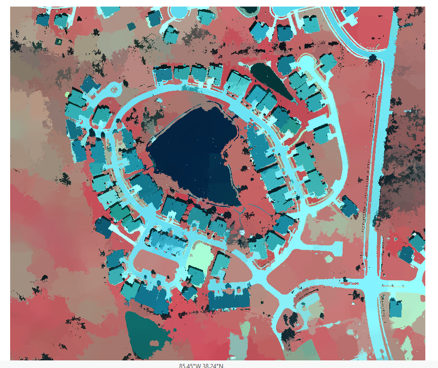Then I created values to display the vegetation health as shown in Map 1. The False color IR uses the higher spectral bands within the Red, Green, and Blue to be changed. I used Red as Band 5, Green as Band 3, and Blue as Band 2. With this I created a map showing the False color IR values of the vegetation in this area (Map 2).

Figure 5. Image Analysis window that is highlighting the NDVI leaf selection under "Processing"

Map 4 brings in the skills and knowledge from the previous lab on how to obtain permeable and impermeable surface data.First, extracting the spectral bands will be used to distinguish urban features from natural features. The tool used here is the "Extract Bands" to create a new image with only three bands. Here the three bands for the false color IR will be bands 5, 3, and 2 in that order so that the vegetation shows up red and the roofs and roads appear darker green to gray. Next, requires using the Segment Mean Shift tool (figure 6). This tool makes it easier to classify the image. After the image becomes easy to classify, the Image Classification tool is used to label the differences in vegetation, roads, driveway, and roof (figure 7). After saving the classification, the next tool to use is called "Train Support Vector Machine Classifier" (figure 8). This tool creates a raster and allows you to classify the features the way you want. After the classified raster is completed, the coded values of 0 (impermeable) and 1 (permeable) are inputted to distinguish between the impermeable surfaces (house, driveway, roads) and the permeable surfaces (yard and fields).

Figure 6. Segment Mean Shift tool window for inputting the RGB image.

Figure 7. The training sample manager allows you to group similar classes together such as similar vegetation, roads, driveways, or roofs

Figure 8. Train Support Vector Machine Classifier tool window

Results

The first map shows the regular RGB image with bands 3, 2, and 1 all placed in the correct spectral band placement. The lower second and third maps display a significant pattern with the vegetation having a bright green to yellow color within the NDVI map and a red to pink color in the False color IR map. The roads and house however display a bright orange to yellow color in the NDVI map while the False color IR map is a dark green to bright blue. The fourth map reveals the difference between the permeable and impermeable layers in the area of interest. Through the process of creating the fourth map however there was some difficulties so the car in the driveway and a small spec of the driveway seem to show as permeable however we know this is untrue.

Map 1. RGB image of the Fall Creeak area of interest

Map 2. NDVI map of the Fall Creek area of interest

Map 3. False color IR map of the Fall Creek area of interest

Map 4. Map of the Fall Creek area of interest Permeable vs. Impermeable layers

Adding GCP's to Pix4D

Introduction

In Pix4D software, ground control points (GCP’s) are used to align the image with the surface of the earth so that your resultant products are spatially and geographically accurate. GCP’s are first collected out in the field from a GPS system with images that have specific coordinates tied to them. The reason we use GCP’s in Pix4D software is to enhance the spatial context of the data, allowing the final products to be more geometrically accurate than the raw data collected with the GPS system.

Methods

In this lab GCP’s have already been obtained from the field and imported onto the computer so that they can be used on the images provided from the Litchfield flight logs. Therefor moving tying down the GCP’s in Pix4D is what will be discussed in the section below. Since last week was getting familiar with Pix4D and how to process images, we will now use GCP’s to further enhance the accuracy of the images, process those enhanced images, and have a more geospatially correct final product.

First, when opening up Pix4D, name the project with the specified characteristics of the project. Then create a workspace in which you can keep all your data saved in as shown in figure 1. On the next page, add the images of the flight you want and make sure the “Shutter Model” is set to Linear Rolling Shutter.

Figure 1. Showing the new project window with the name and desired workspace

Next step is to import GCP’s by clicking on the “Import GCP's…” in the GCP/MTP Manager. When adding GCP’s you have to make sure your latitude and longitude numbers are correct. Y corresponds with latitude, and X corresponds with longitude (figure 2). If the latitude and longitude numbers are reversed, your data will be thrown way off and the images will not line up spatially correct. If it’s correct, the GCP’s will show up in your flight area.

Figure 2. GCP/MTP Manager window with the Import GCP coordinate window popped up.

After all the information is correct and GCP’s are imported, run the initial processing because tying the GCP’s to the imagery is way easier and more efficient in rayCloud rather than doing it manually. Make sure you uncheck steps 2 and 3, then you can press start to run the initial processing (figure 3).

Once the initial processing is finished, go into rayCloud editor and click on a GCP point to bring up the images where that GCP is located. Find the GCP within the image and click on the center to tie the image down to the GCP (figure 4). For each GCP, use 2 to 3 points in order to tie down the image. Once the GCP’s are tied down, go to “automatic marking” and “apply.” Next, go under “Process” and select, rematch and optimize.

Figure 3. Showing where to check step 1, uncheck steps 2 and 3.

Figure 4. Picture showing where the images are tied down to the GCP's in rayCloud.

Since there are two sets of data that need to be put together, the merge project selection must occur at the first window instead of selecting new project. This allows the processing of each dataset to happen faster. After the projects have been merged, the finished product can be used in ArcMap to make maps.

Results

The new DSM can now be brought into ArcMap in order to view all of the data and to create various maps. The map I have created below in figure 5 is an elevation map of Litchfield that also shows all of the ground control points (GCP). Since these GCP’s have been added, this new map is more accurate than the map created in the first Pix4D lab.

Figure 5. Map created from Pix4D Litchfield Flights 1 and 2 data.

Conclusion

Collecting GCP’s and using them as tie down points with the imagery can greatly increase the accuracy of your maps. This is a great way to ensure the accuracy with UAS platforms and collect more accurate data such as volumes within the Pix4D software. Merging two projects also is great to create a larger connected map that’s within the same location.  

Value Added Data Analysis with ArcGIS Pro

Introduction

ArcGIS Pro will be used through an online tutorial through Esri and I will be calculating impervious surface area. This tutorial will allow me to classify an aerial image to determine surface types.

Methods

Lesson 1. Segment the Imagery

First, download the data into the designated folder for saving purposes and open an aerial image into ArcGIS Pro. This map is a neighborhood near Louisville, Kentucky and has 6-inch resolution, and is a 4-band aerial photograph. Next you will open up the tasks folder under the project pane in order to get the steps on how to calculate surface imperviousness (figure 1).

 Figure 1. Project pane showing where to open up the tasks window

Next to do is extracting the spectral bands while setting specific parameters to create a new image with only three bands. Then I clicked create new layer down at the bottom and a layer with three bands extracted is shown on the map (figure 2).

Figure 2. Extracted spectral bands of the new layer

Next is segmenting the image where you’ll group similar pixels into segments. First I clicked the segment mean shift raster function and input all the correct parameters and once again click create new layer. This will enable the image to be simplified and classify broad land-use types more accurately (figure 3).

Figure 3. Segmented image where it has been simplified

Lesson 2. Classify the Imagery

Right away I cannot create the training samples in ArcGIS Pro so ArcMap must be opened and the training samples are exported to a shape file of your desire. First connect to the desired folder in ArcMap and turn on Image Classification toolbar to create training samples. Bring into ArcMap the Louisville Segmented and Louisville Neighborhood images and makes sure the Louisville Segmented is in the Image Classification Layer. Next select the Training Sample Manager to open up the window as shown in figure 4.

Figure 4. Training Sample Manager window

Next I created seven classes of types of land use in the image by merging multiple colors of the same class into one. These classes consisted on Gray Roofs, Roads, Driveways, Bare Earth, Grass, Water, and Shadows (figure 5). Once the seven classes were finished, I saved the training samples as a shapefile into my designated folder.

Figure 5. Classifying each type of land use (Gray Roofs was the first class)

Next I went back to ArcGIS Pro and opened up the train the classifier task. The parameters window opens up and you input the raster and training sample file while saving it to the correct place (figure 6). Once the parameters are all correct, click finish and go on to classifying the imagery.

Figure 6. Train the Classifier parameters window

Go to Classify the Imagery in the tasks pane and input the parameters. After the parameters are set, run the tool and a map with those color classes are created. Next you change the value of the fields by inputting 0 for gray roofs, driveways, and roads while bare earth, grass, shadows, and water are set to 1 (figure 7).

Figure 7. Value of the fields are changed to 0 (impervious) and 1 (pervious)

Lesson 3. Calculate Impervious Surface Area

In this last lesson, an accuracy assessment on the classification to determine if it is within an acceptable range of error will be performed. After that includes calculating the area of impervious surfaces per land parcel so the local government can assign storm water fees.

First, create accuracy assessment points by going under the tasks pane and selecting the correct inputs and click run. After its run, open up the attribute table in the contents pane under My Accuracy Points. This shows all of the fields that the points have on the map (figure 8). Then for the first ten accuracy points you’ll change the GrndTrth to either a 0 or 1, whatever the class it falls into on the map. After that is finished, Click run, Save edits, and Finish the task.

Figure 8. Table of My Accuracy Points

Next is compute a confusion matrix using the points from before.  Again you’ll click the task of Compute Confusion Matrix, input the parameters, and Finish the task. This shows the ability to give an estimate on how accurate the data truly is (figure 9).

Figure 9. Table which shows the accuracy of the point data

After that is completed close the table and open the Tabulate the Area task. Input the correct parameters and run the tool. Once the new table is created, a table join with parameters must be filled out as well in order to join the tables together. Once the parameters are entered, hit Finish and the tools run and the task ends.

Lastly, the parcels need to be symbolized by impervious surface area to depict the area attribute on the map. First, Click the Clean up the table and symbolize the data task and select the Parcels layer, then click run. Edit the names in the correct rows and columns as shown in figure 10.  

Figure 10. Parcel layer attribute table that has been edited

Following the edits, Run the Parcels layer by making sure it is checked and highlighted in the Contents tab before running. Then set the correct parameters in the symbology tab to the right side of the project. The symbology of the map shows that the highest area of impervious surfaces appear to red and the low area of impervious surfaces appear to be yellow (figure 11).

Figure 11. Symbology map of the most impervious parcels to the least impervious parcels

Conclusions

In this lab I classified an aerial image of a neighborhood to show areas that were pervious and impervious to water. Then I assessed the accuracy of my classification and determined the area of impervious surfaces per land parcel.

Processing Pix4D Imagery

Introduction

Pix4D software is used for constructing point clouds that can be turned into orthomosaic images obtained from UAS platforms. This software has numerous applications including agriculture, mining, emergency response, and various others.

Part 1: Get familiar with the product

What is the overlap needed for Pix4D to process imagery?

The recommended overlap for most cases is at least 75% frontal overlap (with respect to the flight direction) and at least 60% side overlap (between flying tracks). It is recommended to take the images with a regular grid pattern shown in figure 1. The camera should be maintained as much possible at a constant height over the object.

Figure 1. Grid pattern of UAS platform taking aerial pictures

What if the user is flying over sand/snow, or uniform fields?

If there is complex geometry or large uniform areas within the overlapping images, it is much more difficult to extract common characteristic points. In order to get good results the overlap between images should be increased to at least 85% frontal overlap and at least 70% side overlap. Also increasing the altitude will provide less perspective distortion and better visual properties.

What is Rapid Check?

Rapid Check is a processing system where accuracy is traded for speed since it is mostly used in the field while obtaining data. It processes faster in an effort to quickly determine whether sufficient coverage was obtained, but the result has low accuracy.

Can Pix4D process multiple flights? What does the pilot need to maintain if so?

Pix4D is able to process images from multiple flights but in order to maintain that the pilot needs to make sure each 1) plan captures the images with enough overlap, 2) that enough overlap between two image acquisition plans (figure 2), and 3) that different plans are taken as much as possible under the same conditions such as weather, time of day, altitude etc.

Figure 2. UAS grid pattern route with enough overlap to process images

Can Pix4D process oblique images? What type of data do you need if so?

Pix4D can process oblique images but it will not create a complete orthomosaic. For this type of data you would need multiple flights with images taken at angles between 10 and 35 degrees. The images should have plenty of overlap in each data set but it is strongly recommended to use GCP’s or Manual Tie Points to properly adjust the images.

Are GCPs necessary for Pix4D? When are they highly recommended?

Ground Control Points are not necessary for Pix4D but the accuracy of the data is dramatically increased when they are used. GCP’s are highly recommended for high precision data and using oblique and nadir images together such as city reconstruction.

What is the quality report?

The quality report is the final report that is automatically displayed after you have processed your data. It gives information on the images, dataset, camera optimization, matching, georeferencing, and other information about the data.

Part 2: Using the Software

In class professor Hupy went through the steps necessary to create a Pix4D project. A PowerPoint was also used to help explain the steps taken throughout.

After the flights have been made and all the data is downloaded onto your computer, open up Pix4D and select Project>New project from the menu bar to open up a New Project window (figure 3). Within this window you must create a name using the date, site, platform, and altitude. Also select a location to save the project in.

Figure 3. New Project window

Click Next and continue with selecting all of the images you want to process and create the point cloud with. Simply select the images out of the folder and import them (figure 4). Then edit the camera model by selecting the “Edit” button under “Selected Camera Model.” Here a new window is displayed and changing the camera properties to Linear Rolling Shutter is done so by clicking “Edit” under “Camera Model Name” and changing the “Shutter Model” to Linear Rolling Shutter (figure 5).

Figure 4. Select the images for processing

Figure 5. Edit Camera Model window and changing Shutter Model to "Linear Rolling Shutter"

Select Next and continue to the Processing Options Template. As shown in figure 6, you can select what type of project you want the software to develop. Here I will be creating a 3D map from the images so the 3D Map option is selected.

Figure 6. Selecting a Processing Options Template, in this case 3D Maps

The last step before processing the data is selecting the desired coordinate system for the project to be displayed (figure 7). In this case the desired coordinate system was already selected so I went ahead and clicked finish to create the project.

Figure 7. Select a desired Output Coordinate System

After clicking Finish, a map view screen appears showing the overall layout of the flight. Right away go to processing steps 2 and 3 and uncheck those, then click on processing options in the lower left corner (figure 8). Press start and go practice on the flight simulator to buy some time because it does take a while to process.

Figure 8. In the lower left corner of the screen, uncheck steps 2 and 3 then click start

Once it is done processing a quality report will provide information on the quality of data accuracy and collection that has been taken (figure 9). The report looks good if all the steps are green and no red errors appear.

Figure 9. Quality Report table 

Next go to RayCloud and turn off cameras and turn on the triangle mesh to view the model (figure 10).

Figure 10. In rayCloud, uncheck the cameras and turn on the triangle mesh located in the contents area

In the dataset 68 of the 68 images (100%) were calibrated and all of the images were enabled. Figure 11 displays the number of overlapping images computed for each pixel of the orthomosaic. The red and yellow areas indicate low overlap with poor results and the green areas indicate an overlap of over 5 images with good quality.

Figure 11. Overlapping images with green having high overlaps and red with low overlaps

Next I measured the volume of one of the piles within the area of interest. First, I clicked on Volumes, then I digitized around the base of the pile and when the last vertex was put in, Right-click and finish the sketch. Then click compute and it gives data for Terrain 3D area, Cut Volume, Fill Volume, and Total Volume as shown in figure 12.

Figure 12. Area of Interest where volume was calculated

The last feature I used in Pix4D was the “fly through animation video.” In order to create this video, click on rayCloud, and go to New Video Animation that is located towards the top. From there I drew out how many timestamps I wanted to create and what direction the video focused on. After the video was created select a folder to save to and select Render. A video has been added below to show the 3D area of Litchfield.

Part 3: Maps

Map 1. Orthomosaic of Litchfield underlain by World Imagery Basemap and with the "No Data" removed

Map 2. DSM of Litchfield with the elevations of the site, red is higher elevations while green is lower elevations