UAS Mission Planning Software

Introduction

This week's lab covers a mission planning software that enables us to utilize the proper steps taken prior to flying the UAS platform. The mission plan is created and allows for the platform to conduct a safe flight in which you define the parameters or mission settings for your specific flight plan. Multiple steps need to be taken not only with your platform and equipment that you are using but also the surroundings that you are going to be flying in. This includes knowing your area of interest, weather, terrain, and any other possible implications to the scene that may alter your flight planning.

Methods

Before you even leave the office there are some key planning essentials that may come back to haunt you if your not aware of the situation you are running into. This includes knowing the area that is being study such as, is the cell signal good, are there lots of people or traffic. Also knowing the vegetation and terrain can make a difference on how your flight plan will go like natural obstacles and land features. Checking the weather is another good observation to take note before leaving the office. Lastly, make sure you have all the right equipment prepared and the batteries are fully charged to get the maximum flight time needed.

When you first get into the field, check again to make sure all of your equipment is with and operational. As far as weather, check for wind, both speed and direction, check the temperature, and check the dew point. Also get an idea of the vegetation around you, this may decide where you want to land the UAS for soft and smooth landing conditions. Another point to add is assessing if there is any EMI issues such as power lines, underground cables, or power stations in the area. Next, get the elevation of the launch site and establish the units in which the team is working in to maintain consistency. Once everything in the surroundings is assessed and seems good to fly, confirm the cellular network is good and bring in the data of your field observations into the pre-flight check and flight log.

Software Demonstration

In this demonstration Bramor's C3P Software is used to easily setup mission parameters out in the field and on the go. Taking a look at the map there are a few symbols that should be known for take-off and landing reasons. There is 4 primary symbols; H - Home, T - Takeoff, R - Rally, L - Landing. The mission settings have 5 parameters that can be set during the pre-flight checklist (figure 1). After the mission settings are set, the Draw tool on the right hand side is used to determine the specified flight route and the 3D map view allows the flight route to be displayed in the flight area with the surrounding terrain in 3D. 

In this software 4 different experimental flight missions were proposed. The first mission consisted of drawing customized waypoints around the Bramor Test Field while experimenting with different side-lap, overlaps, speeds, and absolute vs. relative flying altitudes. These waypoints represent the flight path the UAS will take until the last waypoint is established and it goes into the rally point and landing position (figures 2 and 3). The second flight mission plan is a corridor mission that follows along a linear feature such as a road in the area (figure 4). This corridor flight covers a perfect flight plan that uses the overlap and sidelap parameters in the mission settings so that the area is covered most efficiently. The third flight mission plan took into account some of the terrain in the surrounding Bramor Test Field areas (figures 5 and 6). The larger percentage of overlap in the flight plan there is, the more waypoints the mission planner will establish which makes the flight much longer. A problem that arise is the difference between "absolute" and "relative" altitude. Figure 6 displays a planned mission that makes the UAS fly right into the side of the hill (absolute altitude) and a planned mission that follows topography (relative altitude). Obviously in this case relative altitude is chosen so the UAS follows topography and does not crash into the hillside. The last mission was customized mission plan which was located in the backyard of a childhood home of mine (figures 7 and 8). This route flies on both sides of the a river that is excellent for fishing. Unfortunately when I first created the flight plan I didn't realize there were so many tree's right next to the river.

Figure 1. The Mission Setting parameters for pre-flight.

Figure 2. Waypoint flight plan with custom waypoints, home, takeoff, rally, and landing

Figure 3. 3D view of the custom waypoint flight plan in ArcGIS Earth

Figure 4. 3D view of the mission corridor flight plan along the nearest road with the takeoff and landing points represented very well near the left hand side of the image

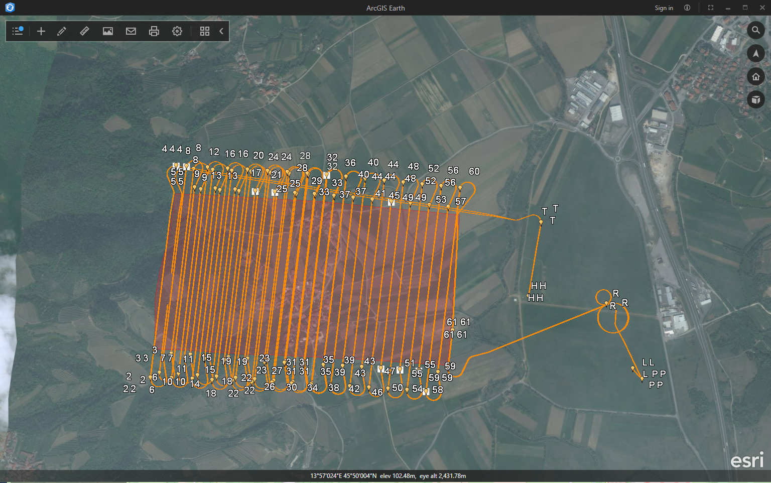
Figure 5. Plan view of a flight plan with some elevation increase on terrain towards the left side of the image.

Figure 6. 3D view of the terrain flight plan displaying an "absolute" altitude mission (goes into the hill) and a "relative" altitude" mission (follows topography).  

Figure 7. Plan view of a customized flight plan of the river near a childhood home.

Figure 8. 3D view of the customized flight plan created near a childhood home.

Mission Planning Essentials Review

The importance of going through numerous steps before the UAS is in the air can be arguably just as, if not more important than the actual flight. Without the pre-flight checklist and mission planning essentials the data cannot be collected nearly as easy or as efficiently. The great part about this program is that the mission settings and parameters make it very user friendly and understandable. One of the neatest parts I thought is with different terrain you can determine whether you have an "absolute" altitude or a "relative" altitude. Another great integration is the ability to bring up your flight plan into ArcGIS 3D. Also having certain icons flash at you lets you know what you are missing before you can take flight which I believe is pretty important.  An issue that I thought was difficult to deal with is the duration of the flight path simulation. I didn't seem to find any glitches or spots that were really standing out or lacking in. Overall this program was pretty great to use and seems like an awesome mission planning software.

Processing and Annotating Oblique Imagery

Introduction

The lab this week consisted of taking oblique imagery from a UAS platform that flew in a corkscrew fashion around an object and annotating the images to receive a better quality 3D model for the finished product. In the previous projects we have used nadir format meaning the picture was taken looking straight down at the ground. An advantage of oblique imagery is the display is more representative of what the human eye sees at the surface. The three different objects that were captured in this project was a front-end loader, a shed, and a truck. The first experiment will include using 3D modeling without image annotation and comparing it to 3D modeling with image annotation. The image annotation in this project for 3D modeling is supposed to eliminate unwanted background content so that the 3D model is not distorted by those surrounding objects in the background.

Study Area
The study area included a front-end loader at the Litchfield mine site. The background consisted of pretty much all sand. The shed and the truck were both done at the South Middle School in Eau Claire. The shed has the sky, trees, and a running track in the background. The truck has the parking lot and some grass in all of its background. For all three of the locations, the images appeared to have been taken mid day because there are hardly any shadows other than the shed which may have been done in the evening.

Methods
The first part of the lab was to copy all of the oblique imagery into our own folder. Before starting on the project in Pix4D, as you go through and select the correct the images you want for the project, at the "Processing Options Template" you want to select the "3D Models" template as shown in figure 1.

Figure 1. 3D Model template option in a new project

The next step is to start processing the images WITHOUT doing any annotation on the images. On this part I selected the front-end loader to process and compare without annotating images. After the processing was done, a video animation of the 3D model was the best way to represent the final product. In order to get a video animation, first you start by selecting the "New Video Animation" button in the Create tab. Next you setup your camera angles to portray the best possible angles of the 3D model. Each angle that is desired should be used by selecting "Record Trajectory Waypoint." after the waypoints are selected and finished, slect the parameters you want for the final output as shown in figure 2. So the video animation of the 3D model without annotating the front-end loader images is shown in the video below.

Figure 2. Trajectory waypoints for a video animation of the 3D model

Front-End Loader without annotation.

The next part is to annotate some of the oblique imagery with the "Image Annotation" tool. Annotation on the images is used to remove an object that appears in some of the images such as the sand in the front-end loader images, the trees within the shed images, or the grass and blacktop in the truck images. First off, select the image you want to annotate by going into Cameras > Calibrated Cameras > and select an image. Over on the right hand side, the image will appear and a tool that looks like a pencil is the "Image Annotation" tool (figure 3). For annotating, the Mask setting was used to highlight the background in all of the images that were annotated (figure 3). Once that is selected the tedious work highlighting of the background can begin. After about 8 images were annotated on the front-end loader, select the processing steps 2 and 3 to recreate the 3D model with annotated images. The final product can be seen in the video below.

Figure 3. The window that is displayed while annotating the selected image from the left hand side

Front-End Loader with annotation.

The next two projects with the shed and the truck in the parking lot consisted of the same exact workflow. Each projected had about 6 to 8 images annotated at different angles to get the best quality out of processing the 3D model for the final product.

Results
For the results of comparing the front-end loader with and without annotating some of the images was pretty minute. Some of the areas that may have been affected for the better were areas with gaps or holes to see the background such as the hydraulic hoses in the front, or near the muffler in the back. Otherwise the 3D model did not have much differences. Also on the front-end loader, the bucket was distorted and looked like it had something in it when the images show different.

The middle school shed honestly turned out pretty bad as far as getting rid of background objects and distortions. The peak of the roof has a white to light green and blue bubble like figure across the top. I'm assuming this may have to do with all of the objects in the background such as the trees and sky that make it difficult to produce the 3D model. Also the one wall on the shed was distorted and appeared to go through the roof which obviously is impossible. The fly through animation can be seen in the video Middle School Shed Annotated

The truck 3D model turned out probably the best as far as quality goes. the parts that got distorted were areas underneath the truck and the windows of the truck. This may have turned out the best because the only background that needed to be annotated was the ground which is completely flat all around the truck. The fly through animation of the truck can be seen in the video Truck Annotated.

Discussions
The oblique imagery in the project is very helpful in processing a 3D model of an object. However, when it came to annotating the images so that any background noise can be ignored was a very tedious task. When looking at the front-end loader images, the sand with tracks in it made it difficult for the sand to be masked as a whole. The worst one to annotate though was the truck in my opinion. the reason is because when annotating the blacktop parking lot, the pixels hardly ever match so you are even more tedious with masking the background. The easiest annotating was in the shed with the sky as the background. The similar pixel color of the blue sky made it so large chunks of the sky could be annotated with one click.
In order to get the best quality with annotating images to get a better 3D model would probably be to select images at different angles rather than multiple images from the same angle. This allows for the surroundings in the image to make the focused object to become less distorted. I feel like this may have been one of my problems when it came to the final 3D model of the middle school shed. I simply didn't pick enough different angles to annotate.

Calculating Volumes using Pix4D and ArcMap

Introduction

This lab consists of calculating volumes of stockpiles in both Pix4D and ArcMap using the Litchfield data from a previous lab. In the lab there are three different methods on how to calculate the volumes of stockpiles with different software. The first will be using Pix4D, then ArcMap with Raster Clip, and ArcMap with TIN. This is a very quick and efficient way of calculating the leftover stockpiles in mines, quarries, or other related applications.Using the UAS is also very accurate, detailed, cost effective, and time efficient for whomever is wanting to obtain the volumes of stockpiles.

Operations Utilized

Raster Clip - The clip is a data management tool that allows a portion of a raster dataset to be cut out of the original feature dataset.

Raster to TIN - Raster to TIN is a 3D analyst tool that converts a raster into a triangulated irregular network (TIN) dataset.

Add Surface Information - Add surface information is another 3D analyst tool that produces attributes to features with spatial information deriving from a surface.

Surface Volume - Surface Volume is a 3D analyst to that calculates the area and volume of a refion between a surface and a reference plane.

Polygon Volume - Polygon Volume is a 3D analyst tool that calculates the volume and surface area between a polygon and terrain or TIN surface.

Cut Fill - Cut fill is a 3D analyst tool that calculates the volume change between two surfaces. This tool is typically used for cut and fill operations.




Methods

Pix4D stockpile volume calculations

Starting this lab will consist of creating a new folder for the Litchfield data and copying that data to the new folder. This process will take a fair amount of time because of the large amount of data being copied over. After the Litchfield map is opened up in Pix4D, the first place to go is to the volumes tab on the left hand side of the project. Next select the "add volume" button to add the 3 different stockpiles. After it is selected, you can start digitizing your 3 stockpiles by digitizing around the base of each stockpile as shown in figure 1. After the digitizing is done, select calculate to get the volumes of the stockpile which is also shown in figure 1. The stockpile to the far right has an estimated volume of 978.60 cubic meters, the middle pile is 527.37 cubic meters, and the smallest pile up top is 16.13 cubic meters.

Figure 1. Pix4D area of all 3 stockpiles used for volumetric analysis

ArcMap raster clip stockpile volume calculations

First part of this method is to open the mosaic that was from Pix4D and create a new geodatabase with 1 feature class for each individual stockpile. Next step is to digitize the three piles by using the Extract By Mask tool with the correct parameters for each individual pile as shown in figure 2.

Figure 2. Extract by mask tool with the parameters for stockpile 1

Next, use the surface volume tool to calculate the area and volume of each stockpile with the correct parameters as shown in figure 3. In order to find a reference plane use the identify tool to get information on the surface elevation on each stockpile given by the pixel value field. After the tool is ran, an attribute table is created with values of plane height, area, and volume as shown in figure 4. In figure 5, model builder is shown how to use the tools for stockpile 1. This can be used for the other two stockpiles as well.

Figure 3. Surface volume tool inputs

Figure 4. Attribute table after the surface volume tool is ran

Figure 5. Data flow model of stockpile one using raster clip

ArcMap TIN stockpile volume calculations

The first step to finding the volumes as a TIN, you must convert the three raster clips into a TIN of course. This is done using the Raster to TIN tool as shown in figure 6. Now that there are TIN files for each of the three stockpiles, the next tool to use is the Add Surface Information tool with the correct parameters in place (figure 7). The last tool you need to use is the Polygon volume tool to calculate the volume and surface area of the TIN (figure 8). Figure 9 displays the data flow model for the TIN volume calculations.

Figure 6. Raster to TIN tool inputs

Figure 7. Add surface information tool inputs

Figure 8. Polygon Volume tool inputs

Figure 9. Data flow model of the TIN for stockpile

Results

The table below displays the three different calculations used from Pix4D, Raster, and TIN.

Table 1. Results table for volumetric analysis

Map of the Litchfield mine site with the stockpiles used for volumetric analysis

Discussion
In the results it shows that the Pix4D has lower calculations than both the ArcMap Raster and TIN calculations. The Pix4D method was very simple and to the point just by digitizing the base of each stockpile and having the program calculate the rest. With ArcMap Raster and TIN calculations however multiple tools needed to be use correctly with the correct parameters inputted.